Table of Contents
- 1 What is Perfect Competition?
- 2 Definition of Perfect Competition
- 3 Assumptions of Perfect Competition
- 4 Demand Curve under Perfect Competition
- 5 Firm Equilibrium Under Perfect Competition
- 6 Short Run Equilibrium Under Perfect Competition
- 7 Long Run Equilibrium under Perfect Competition
- 8 Conclusion
What is Perfect Competition?
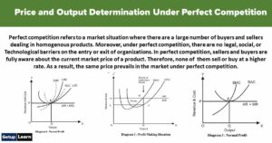
Perfect competition refers to a market situation in which there are a large number of buyers and sellers of homogeneous products. The price of the product is determined by industry with the forces of demand and supply.
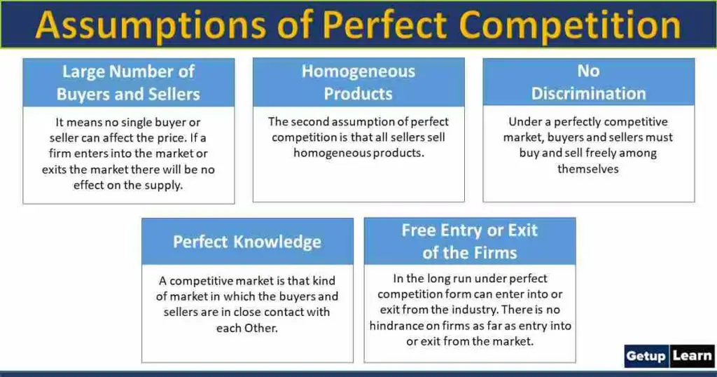
Table of Contents
For instance, if we require a pen there should be several shops selling pens. Under conditions of perfect competition, every seller should be selling the same quality of pens at a uniform prevailing price in the market. We may buy a pen from any shop at the price of rupees 10.
If another shopkeeper charges rupees 12 for the same quality of pen, nobody will buy from him but if A shopkeeper charges rupees 9 all will buy pens from that particular shop. But both situations are unrealistic. There must be one price prevailing throughout the market.
Perfect competition is a phrase used often in everyday discussions, and many people have an intuitive and vague understanding of what it means. The concept of Perfect competition is very old and was discussed in a casual way by Adam Smith in his Wealth of nations.
Edge worth was the first to attempt a systematic and rigorous definition of perfect competition. The concept received its complete formulation in Frank Knight’s book, Risk, Uncertainty and profit (1921). Perfect competition is a market structure characterized by a complete absence of rivalry among individual firms.
Thus Perfect Competition In economic theory has a meaning diametrically opposite to the everyday use of this term. In practice, businessmen use the word competition as synonymous with rivalry. In theory, Perfect competition implies no rivalry among firms.
Definition of Perfect Competition
[su_quote cite=”Mrs Joan Robinson”]Perfect competition prevails when the demand for the output of each producer is perfectly elastic.[/su_quote]
Assumptions of Perfect Competition
The main assumptions of perfect competition are as follows:
- Large Number of Buyers and Sellers
- Homogeneous Products
- No Discrimination
- Perfect Knowledge
- Free Entry or Exit of the Firms
Large Number of Buyers and Sellers
It means no single buyer or seller can affect the price. If a firm enters into the market or exits the market there will be no effect on the supply. Similarly, if a buyer enters into the market or exits the market, demand will not be affected. Thus no individual buyer or seller can affect the price.
Homogeneous Products
The second assumption of perfect competition is that all sellers sell homogeneous products. In such a situation the buyers have no reason to prefer the product of one seller to another.
This condition is present only when the commodity is a substance of definite chemical and physical composition.,i.e., salt, tin, specified grade of wheat etc.
No Discrimination
Under a perfectly competitive market, buyers and sellers must buy and sell freely among themselves. It implies that buyers and sellers must be willing to deal openly with one another to buy and sell at the market price.
This may be true of one and all that may wish to do so without opening any special deals, discounts, or favours to selected individuals.
Perfect Knowledge
A competitive market is that kind of market in which the buyers and sellers are in close contact with each Other. It means that there is perfect knowledge of the market on the part of buyers and sellers.
It implies that a large number of buyers and sellers in the market exactly know how much the price of the commodity is in different parts of the market.
Free Entry or Exit of the Firms
In the long run under perfect competition form can enter into or exit from the industry. There is no hindrance on firms as far as entry into or exit from the market. In other words, there are no legal or social restrictions on the firm. A large number of sellers can be possible only if there is the free entry of firms.
Demand Curve under Perfect Competition
Demand Curve of a Product Facing a Perfectly Competitive Firm: Under perfect competition,a single price must prevail and therefore the demand curve or average revenue curve faced by an individual firm is perfectly elastic at the ruling price in the market.
Perfectly elastic demand Curve signifies that the firm does not exercise any control over the price of the product but can sell any amount of the product as it likes at the ruling price.
In the graph drawn above, the demand Curve DD and supply curve SS intersect at point E and determine price OP. Now the firm, having no influence over the price, will take the price OP as given and therefore the average-marginal revenue curve facing it will be a horizontal straight line at the level of OP.
When demand increases and as a result price rises to OP’, the firm will now confront the average-marginal revenue curve at the level of OP’. And if the demand decreases and price falls to OP”, the firm’s average-marginal curve will shift below to the level of OP”.
Firm Equilibrium Under Perfect Competition
The marginal cost curve of the firm is U-shaped. Now in order to decide about the equilibrium output of the firm under perfect competition, the firm will compare the marginal cost with marginal revenue.
It will be in equilibrium at the level of output at which marginal cost equals marginal revenue and the marginal cost curve is cutting the marginal revenue curve from below. At this level, it will be maximizing its profits.
Since Marginal revenue is the same as price (or average revenue) the firm will equate marginal cost with a price to attain equilibrium output. We consider the above-mentioned graph for this, in which price OP is prevailing in the market.
PL would then be the demand curve or the average and marginal revenue curve of the firm. It will be seen from the graph that the marginal cost curve cuts average and marginal revenue curve at two different points F and E. F cannot be the position of equilibrium since at F second-order condition of Firm’s Equilibrium, namely, that the marginal cost curve must cut marginal revenue from below at the point of equilibrium is not satisfied.
The firm will be increasing its profits by producing beyond F because marginal revenue is greater than marginal cost. The firm will be in equilibrium at point E or output OM since at E marginal cost equals marginal revenue, as well as marginal cost curve, is cutting marginal revenue curve from below.
Hence, the twin conditions of a Firm’s Equilibrium Under Perfect Competition are:
- MC=MR=Price
- The MC curve must be rising at the point of equilibrium.
Short Run Equilibrium Under Perfect Competition
The short-run means a period of time within which the firms can alter the level of output only by increasing or decreasing amounts of variable factors such as labour and raw materials while fixed factors like capital, equipment machinery etc. remain unchanged.
The fulfilment of the above twin conditions does not guarantee that positive profits will be earned by the firm or not in order to know whether the firm is making profits or losses and how much of the average cost curve must be introduced in the figure.
In the short run, there are three cases of equilibrium that may occur:
Supernormal Profits
In the graph drawn above, on X-axis, Output is taken and on Y-axis, Price and Cost are taken. At the equilibrium output OM, average revenue is equal to ME and the average cost is equal to MF. Therefore, the profit per unit of output is EF, the difference between ME and MF.
The total economic profits earned by the firm will be equal to EF (profit per unit) multiplied by OM or HF( total output). Thus the total profits will be equal to the area HFEP because normal profits are included in average cost, the area HFEP indicates Supernormal or economic profits.
Losses
In the graph drawn above, on X-axis, Output is taken and on Y-axis, Price and Output are taken. Now suppose that the prevailing market price of the product is such that the price line or average and marginal revenue curve lies below-average cost throughout.
This is shown in the above graph where the ruling price is OP’ which is taken as given by the firm. P’L’ is the price Line that lies below the AC curve at all levels of output. The firm will be in equilibrium at point E’ at which marginal cost is equal to price (or marginal revenue) and the marginal cost curve is rising.
The firm would be producing OM’ output but would be making Losses since the average revenue which is equal to M’E’ is less than the average cost which is equal to M’F’. The loss per unit of output is then equal to E’F’ and the total loss will be equal to P’E’F’H’ which is the minimum loss that a firm can make under the given price -cost Situation.
Since all the firms are working under the same cost conditions, all would be in equilibrium at point E’ or output OM’ and everyone will be making losses equal to P’E’F’H’. As a result, the farmers will have a tendency to quit the industry in order to make a search for earning at least normal profits elsewhere.
Shutting Down
If the price falls below the average variable cost the firm will lose its fixed cost plus some of its variable cost, that is, it will make losses greater than the total fixed costs. Under such circumstances, it will be rational for the firm to close down because by suspending production it can avoid losses incurred on variable costs.
We, therefore, conclude that if the firm is not able to cover even its variable cost fully it will shut down even in the short run to avoid unnecessary losses. This is explained by the following graph:
In the graph drawn above, on X-axis, Output is taken and on Y-axis, Price and Cost are taken. Here along with short-run average cost and marginal cost curves, the average variable cost curve is also drawn. When the price in the market is OP1, the firm will be in equilibrium at point R and will therefore produce output OQ.
Since the average cost which is equal to QS is greater than the average revenue or price which is equal to QR or OP1, the firm will be making losses equal to P1RST. But it will be in the interest of the firm to continue producing at point R because the price OP1 or QR is greater than the average variable cost which is equal to QB.
By operating at price OP1, the firm is covering total variable costs (area OQBA) and a part of fixed costs (area ABRP1). The part of the fixed costs equal to area P1RST is not being covered. The firm should operate and bear the losses equal to P1RST because by closing down in the short run the firm will have to bear the losses equal to the whole fixed costs, the area ABST.
Thus the losses will be smaller in case the firm is working than if it stops producing. If the price in the market happens to be OP2, the firm will be in equilibrium at point D. Price is equal to the average variable cost. At point D the firm is covering the variable cost fully, but it is not meeting any part of the fixed cost.
Therefore its losses are equal to the whole fixed cost equal to the area P2DUV. Even if the firm stops operating, its losses will be equal to the whole fixed cost, therefore it will be a matter of indifference for the firm to operate at price OP2 or not. But if the price falls below the average variable cost for OP2, for instance.
if the price falls to OP3, the firm will simply shut down since the firm will not cover even its variable cost fully therefore the firm will suspend production at price OP3 or any other price below OP2 and will wait for some good time to come.
Long Run Equilibrium under Perfect Competition
The long-run is a period of time that is sufficiently long to allow the farmers to make changes in all factors of production. In the long run, all factors are variable and none are fixed. Firms in the long run can increase their output by changing their capital equipment.
Besides, in the long run, new firms can enter the industry to compete with the existing firms. For a perfectly competitive firm to be in long-run equilibrium, the following two conditions must be fulfilled:
- Price = Marginal Cost
- Price=Average Cost
Hence, the above-mentioned conditions can be amalgamated as follows:
Normal Profit
The case of Normal Profit can be elaborated by the following graph:
In the graph drawn above, on X-axis, Output is taken and on Y-axis, Cost and Revenue are taken. The firm cannot be in the long-run equilibrium at a price greater than OP as shown in the figure.
This is because if the price is greater than OP then the price line would lie somewhere above the minimum point of the aver cost curve so that the marginal cost and price will be equal where the firm is earning supernormal profit since there will be a tendency for new forms to enter and compete away this supernormal profits.
The firm cannot be in long-run equilibrium at any price higher than OP. Likewise, the firm cannot be in long-run equilibrium at a price lower than OP. If the price is lower than OP, the average and marginal revenue curve will lie below the average cost curve so that the marginal cost and price will be equal at the point where the firm is making losses.
Therefore, there will be a tendency for some of the firms in the industry to go out with the result that price will rise and the firms left in the industry make normal profits.
We, therefore, conclude that the firm can be in long-run equilibrium under perfect competition only when the price is at such a level that the horizontal demand curve(AR curve) is tangent to the average cost curve so that price = average cost and firm makes only normal profits..
It should be noted that a horizontal demand curve can be tangent to a U-shaped average cost curve only at the latter’s minimum point. Since at the minimum point of the average cost curve the marginal cost and average cost are equal, price in long-run equilibrium is equal to both marginal cost and average cost.
In other words, the double condition of long-run equilibrium is fulfilled at the minimum point of the average cost curve.
Conclusion
From the above-detailed analysis, we got to know about the description of the “Perfect competition” market structure. Though this market form does not exist in actuality, it gives a very clear idea of the ideal market form that helps in the study of real market structures like Monopolistic Competition and Oligopoly later on.