Table of Contents
What is ISO Product Curve?
An iso product curve is a locus of various combinations of two factors of production giving the same level of output and a producer is indifferent to each of such combinations. All the combinations of two inputs give the same quantum of output to a producer and the producer is indifferent to each combination. He does not have any preference. These iso-product curves are also called production indifference curves. The concept of the iso-product curve is also called production indifference curves.
When all the factors of production are changed in the same proportion then the change caused in the production is called returns to scale. The long run production function is analysed by a new technique known as the ISO-quant or ISO-product or equal product curve.
Iso Quant Schedule
The concept of iso product curve can be explained with the help of iso-quant schedule and diagram:
An iso-quant schedule shows different combinations of two factors of production at which a producer gets the equal level of output is called an iso quant schedule. The schedule is given below:
Iso-quant Schedule
| Combination | Factor A (Labour) | Factor-B (Capital) | Output (Q) |
| A | 1. | 20 | 100 units |
| B | 2. | 15 | 100 units |
| C | 3. | 11 | 100 units |
| D | 4. | 8 | 100 units |
| E | 5. | 6 | 100 units |
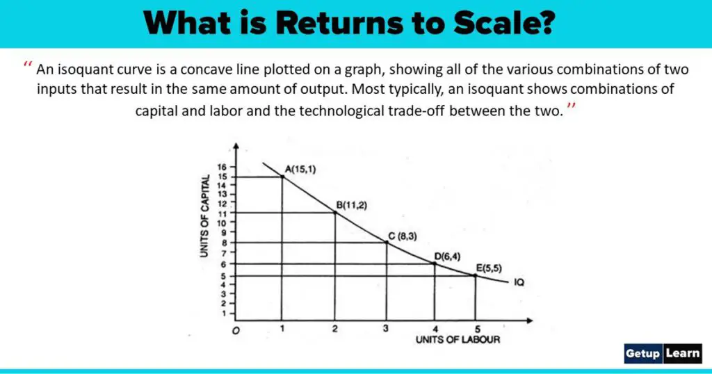
The above schedule shows the different combinations of two inputs namely labour and capital and the resultant output of 100 units from each combination. The units of labour are increasing and units of capital are decreasing but the quantity of output remains the same. The schedule can be shown in the form of a diagram given below:
Iso-quant Schedule Diagram
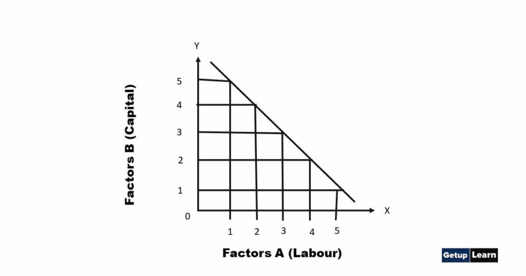
The lP curve slopes downward to the right, It explains with the increase in the units of factor-A and reducing the units of factor-B.
Characteristics of Iso Product Curves
The following are the characteristics of iso-product curves:
Iso-product Curves Slope Downward to the Right
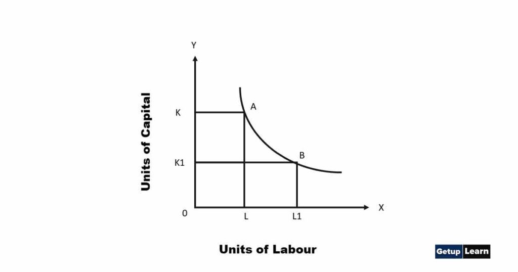
Iso-product curves slope downward to the right because the producer has limited resources with alternative uses and he is faced with the problem of choice. He cannot increase the amount of labour and capital. If he employs more labour he has to employ less capital in order to get the same level of output as given in the following diagram No. 6.
The diagram shows that units of labour are shown on ox-axis and units of capital on oy-axis. A combination shows OK of capital and CL of labour while at B combination OK1 of capital and OL1 of labour showing the same amount of output (100 units). But the producer has employed more of labour and less of capital and on account of it the iso-product curve slopes downward to the right.
Iso-product Curves Are Convex to the Point of Origin
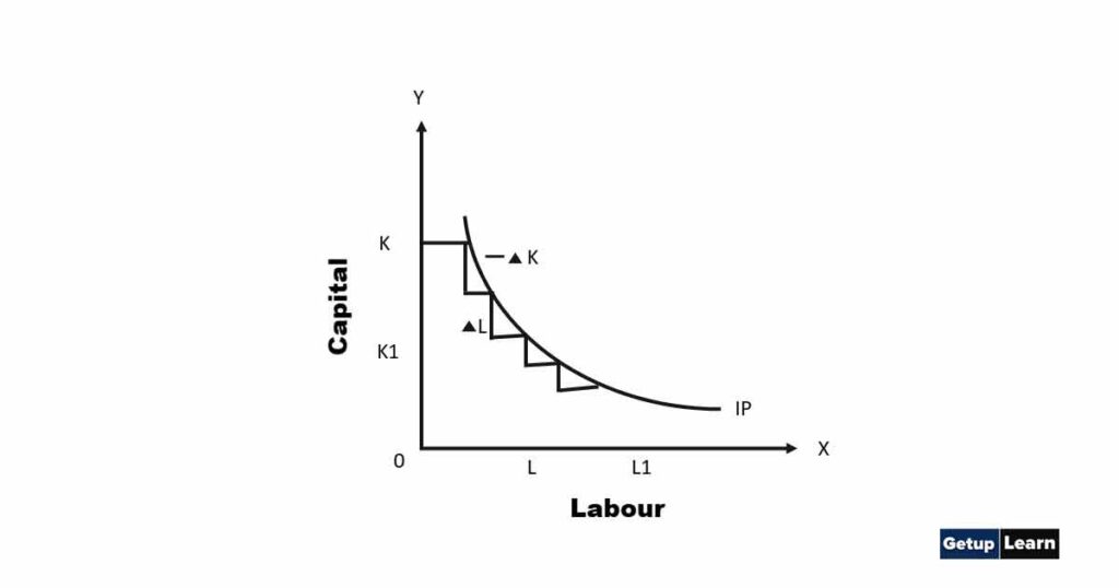
As an indifference curve is convex to the origin. similarly, an iso-product curve is also convex to the origin. In an iso-product curve, a factor of production is substituted by another factor of production and consequently, the marginal rate of technical substitution of labour for capital (MRTSLK) declines and on account of decreasing MRTLK the iso-product curves are convex to the origin. It is shown by the following diagram:
| Combination | Labour (L) | Capital (K) | MRTS LK |
| A | 1 | 20 | – |
| B | 2 | 15 | 5 |
| C | 3 | 11 | 4 |
| D | 4 | 8 | 3 |
| E | 5 | 6 | 2 |
The table reveals that we are increasing the units of labour and reducing the units of capital. The MRTS LK shows a declining trend.
Two Iso-product Curve Never Intersect Each Other
Another characteristic is that two iso-product curves do not intersect each other as different iso- product curve shows a different level of output. It is shown by the following diagram:

Capital and labour are shown on the oy-axis and ox-axis respectively. IP and IP1 are two iso product curves. E is the point where IP and 1P1 intersect each other. Before E point IP is higher than 1P1 and after E point IP1 is higher than IP. In such a situation it is difficult to know which Iso-product curve gives a higher level of output. Hence we can say that it is indeterminate and two iso-product curves do not intersect each other.
Higher the Iso-quant Curve Higher is the Level of Output
A producer gets the same level of output with different combinations of two inputs on the Iso-product curve. But in the case of a different Iso-product curve, the level of output differs. Higher the Iso-product curve higher the level of output and the lower the Iso-product curve lower will be the level of output. It is shown in the following diagram:
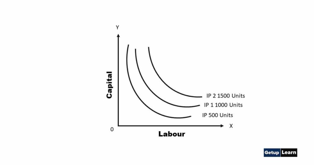
The diagram shows Iso product map in which three Iso-product curves are showing different levels of output. IP, 1P1 and 1P2 are showing 500 units 1000 units and 1500 units respectively which show increasing trends. The higher the Iso-product curve higher is the level of output (IP1 to IP2), lower the iso- product curve lower will be the level of output (IP1 to IP). The highest iso product curve is IP2 and the lowest iso-product curve is IP.
Marginal Rate of Technical Substitution
The marginal rate of technical substitution is an important concept in the study of Iso-product curve analysis. The marginal rate of technical substitution is the rate at which two factors of production (inputs) are substituted. For example, we have two factors of production capital and labour.
The marginal rate of technical substitution of labour for capital (MRTSLK) is the rate at which one unit of labour substitutes the number of units of capital. The MRTSLK can be studied from the following table:
Marginal Rate of Technical Substitution
| Combination | Factor A (Labour) | Factor B (Labour) |
Marginal rate of technical Substitution of A for B (MRTSAB) |
| A | 1 | 12 | — |
| B | 2 | 8 | 4:1 |
| C | 3 | 5 | 3:1 |
| D | 4 | 3 | 2:1 |
| E | 5 | 2 | 1:1 |
The table reveals that all the combinations of factor A (labour) and factor B (capital) give the same level of output. If he has an A combination then 1A+12B will give the same level of output when he employs 5 units of A and 2 units of B (5A+2B) at the E combination the level of output remains unchanged. Hence the marginal rate of technical substitution of factor A for factor B can be written mathematically in the following formula.
Generally, the MRTS declines because as we employ more of factor A then we have to employ less of factor B. It is called the MRTS and each iso-product is convex to the origin on account of declining MRTS. As we know that different combinations of two inputs give the same level of output which is shown by an iso-product curve.
The higher the iso-product curve higher will be the level of output. A producer is faced with the problem of choice because his resources are limited and they have alternative uses. The
choice of producer depends upon the resources at his disposal and the factor prices. An iso-cost curve shows the various combinations of two inputs (labour and capital) that can be employed by a producer with his given resources. It means the resources of a producer and prices of two inputs are shown by this curve.
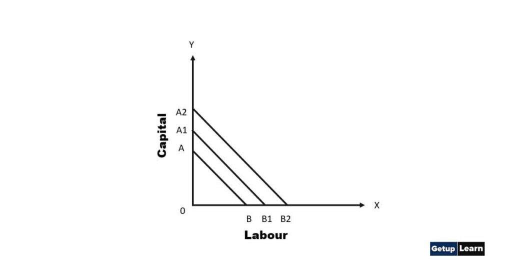
It is given in the diagram. In the diagram labour and capital are shown on the x-axis and ox-axis respectively. AB, A1 B1 and A2B2 are iso-cost lines or curves showing different combinations of labour and Capital. If the producer wants to employ more labour and less capital then he should keep in his mind his budget and the prices of both these factors Higher the iso-cost curve higher will be the need for resources. The iso-cost curve is also known as the outlay line and factor cost line.
Producers Equilibrium Least Cost Combination of Inputs or Factors
A producer has assumed a rational human being. His aim is to maximise his total production by attaining a least-cost combination of factors of production (inputs). Thus a producer will be in equilibrium when a producer gets a given amount of output with the least cost combination of factors of production.
He has several alternatives to produce a given amount of output but he will choose that combination by which he attains optimum factors of production in such a way that he minimises the per-unit cost of production. Iso-product curves help a producer to attain an optimum or least-cost combination of factors of production.
A producer‘s equilibrium can be attained with the help of two tools namely:
- Equal or Iso-product map
- Iso-cost or equal cost curve
An individual firm or a producer attains the optimum combination or least-cost combination of two factors of production where iso- cost curve is tangent to the iso-product curve. It can be explained with the help of the diagram.
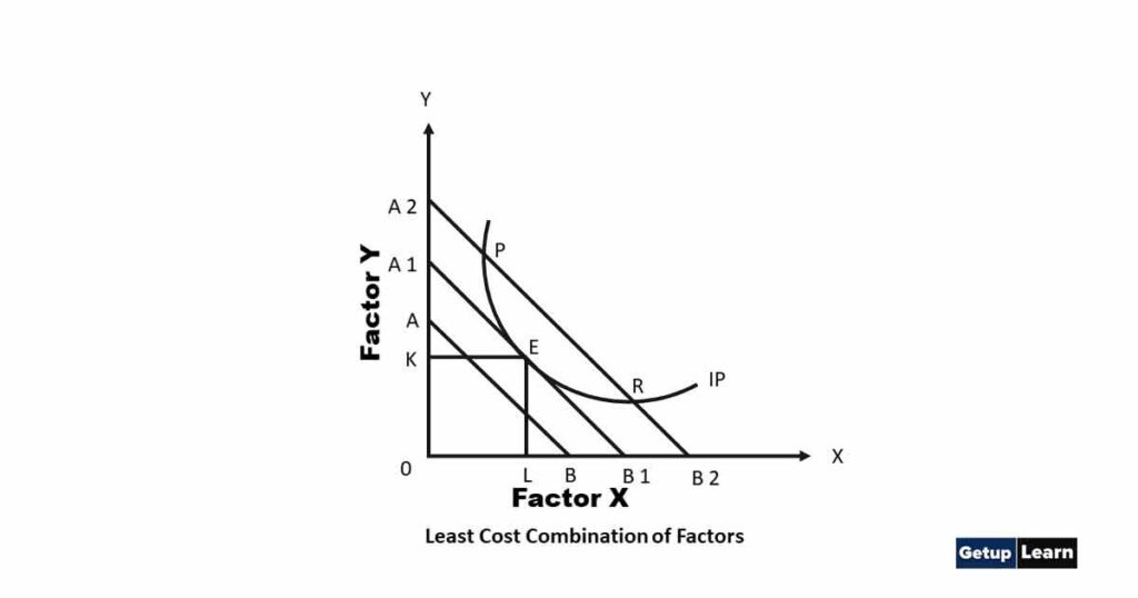
The diagram Shows factor-y on oy axis and factor-X on ox axis. AB, A1B1 and A2B2 are the Iso- cost curves. IP is the iso- product curve on which PER are three combinations, a producer will choose that combination that gives him the least cost.
In the diagram, the least cost combination is E where the cost of production is least or iso product curve touches the A1B1 iso-cost curve. Other combinations (P and R) are on a higher Iso-cost curve. Thus by selecting another combination the cost of production will be higher than that of point E. Hence we can say that with given output, the E combination is optimum which gives least-cost combination for a given amount of output.
What is ISO cost curve shows?
An iso-product curve shows is a locus of various combinations of two factors of production giving the same level of output and a producer is indifferent to each of such combination. All the combinations of two inputs give the same quantum of output to a producer and the producer is indifferent to such each combination.
What is a ISO cost curve?
An ISO-cost curve shows the various combinations of two inputs (Labour and capital) that can be employed by a producer with his given resources.